[IPA 25] How We Matched the Original Hardware – Without Burning Your CPU
- Posted on
![[IPA 25] How We Matched the Original Hardware - Without Burning Your CPU](https://pulsar.audio/wp-content/uploads/jupiterx/images/Thumbnail-IPA25-Video-2-c4eec65.jpg)
So many plugin models lean on simplified math to keep CPU use low.
While that approach works in many cases, it often comes at the expense of accuracy, especially when techniques are applied without regard for the specifics of a given circuit.
More recently, some developers (including us for the Massive) have been turning to SPICE-like circuit solvers and Wave Digital Filters (WDF) to capture full circuit dynamics.
Which brings us to the IPA 25.
The iconic compressor upon which this is based, simply isn’t one where shortcuts or generic methods are an option.
Why This Hardware Compressor Was Different
The hardware upon which IPA 25 is modeled, is not one that can be approximated casually.
It has a strong reputation and its sound is incredibly well known to engineers, so a model that falls short will be spotted immediately.
On smaller or simpler compressors, some developers will try to get away with mapping out parameter combinations into tables and matching each in isolation.
But for the IPA 25, the controls interact much too closely for that approach to work.
And this is a choice that has very real consequences for how the model sounds and behaves.
Why the Modeling Method Matters
Getting this right isn’t only about matching graphs. It’s about making sure the compressor behaves like the original when you actually use it.
That means capturing details like the RMS detection and the program-dependent releases with their specific pre-knee “release-to” voltages.
It also means primarily focusing on what’s audible – to manage our CPU hit as best as possible.
For instance, this is why the op-amp and transformer contributions were modeled at the behavior level – drive, asymmetry, odd/even balance, subtle LF/HF weighting – without brute-forcing an electromagnetic model that would eat two to three times more CPU for little or no mix benefit in this specific model (again the method is chosen on a case-by-case basis).
So in this case, by modeling each module explicitly, we also gained increased flexibility – which allows us to extend the functionality of the original hardware in ways that may have been limited by using another method.
This is how we’re able to include things like parametric sidechain EQ, selectable VCA harmonic modes, an additional clipper/limiter – all without disturbing the original model behavior.
With those priorities set, the next step was to break down the circuit itself and map out exactly how the hardware worked.
Breaking Down the Circuit
So the exploration starts by mapping the full signal and control paths, measuring both static and dynamic behaviors.
The transfer curves, timing laws, and coloration introduced by active and passive stages were all measured and documented.
Luckily, most of these steps were straightforward. So far – so good.
That is, until we got to the Release timing – that’s where things started to become a bit trickier.
In the original hardware, as the release time increases, the compressor shows a slow, program-dependent release that doesn’t really behave in a way that you’d expect.
This was something we really needed to get right, because it’s such a huge part of ensuring that this model doesn’t only “sound” like the original – but it “behaves” like it.
Digging deeper into the release behavior is where we uncovered the most critical detail.
Release Behavior - The Critical Detail
Closer inspection showed that the hardware’s release curve doesn’t behave like a typical exponential or multi-segment release.
As it turns out, at low amounts of gain reduction, the curve bends in a way we’ve yet to see in other compressors – and we’ve been doing this for well over a decade.
None of the standard models came even close – and it was clear that to get this model right, we would need to reproduce this release behavior exactly – and not approximate it with a generic law.
That insight set the direction for the full model: a modular approach where each stage could be measured, recreated, and then assembled into the whole.
It’s this level of detail that we feel makes all the difference in how the final model measures up to the original hardware – and how it behaves when used in real-world mix scenarios.
Building the Compressor Model
So our approach to this one was to first model the machine as a set of independent modules, each measured and expressed in compact mathematical form:
- Drive stages were captured with calibrated waveshaping, tuned to the level-dependent nonlinearities of the hardware.
- Detector path was implemented as a frequency-dependent envelope follower model, matching the gain-reduction behavior observed in measurement.
- VCA and knees were recreated with multi-knee curves to reflect the characteristic transitions.
- Timings were modeled to account for the unusual release, including the way the compressor releases toward a level below the current threshold. This means the unit reacts differently depending on whether the signal drops just under threshold or several dB below—especially evident on SOFT and MED knees.
And then by handling each of these modules independently, each part could be validated directly against measurement.
Only after each module is checked and re-checked against the hardware, do we then put the pieces together into a complete model of the hardware.
So now with the complete model in place, the next step was to see how it compared to the real unit.
Verifying Our Model Against Hardware
Now, once we’ve assembled all the pieces, we begin to compare the full model directly to the hardware in many different ways.
The first of which is verification of things like transfer curves, THD vs. level, step responses, and detector weighting confirmed that the math tracked the hardware closely.
Here are some examples of how the software measure to the original hardware – where GREEN is the hardware and RED is the model.
As you can see, the match is incredibly close…
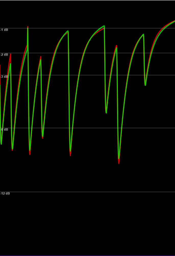
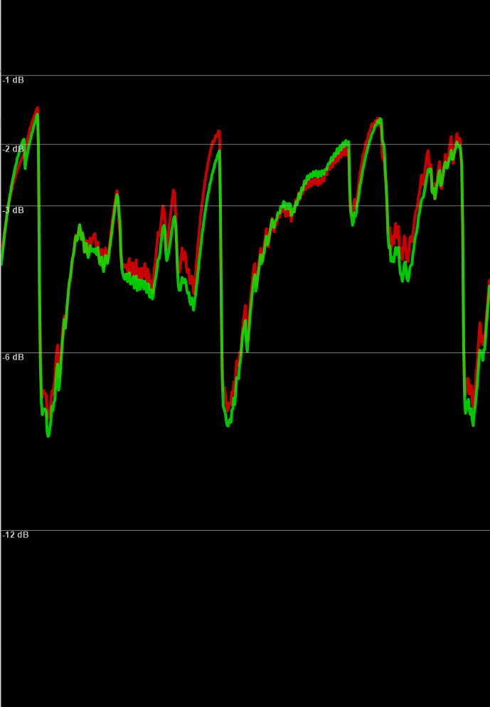
Of course, graphs only tell part of the story.
What matters most is how it sounds…
What The IPA 25 Sounds Like Against The Hardware
Try It Yourself
Now, we get that measurements and A/B files can only go so far.
The true test is how the model behaves in your workflow, on your own material, with the settings and creative choices you make every day.
So, we invite you to try the IPA 25 Multi-VCA Dynamic Processor in your sessions and hear for yourself how it stands up.